Introduction¶

Research on dynamical and hybrid systems has produced several methods for verification and controller synthesis. A common step in these methods is the reachability analysis of the system. Reachability analysis is concerned with the computation of the reach set in a way that can effectively meet requests like the following:

For a given target set and time, determine whether the reach set and the target set have nonempty intersection.
For specified reachable state and time, find a feasible initial condition and control that steers the system from this initial condition to the given reachable state in given time.
Graphically display the projection of the reach set onto any specified two- or three-dimensional subspace.

Except for very specific classes of systems, exact computation of reach sets is not possible, and approximation techniques are needed. For controlled linear systems with convex bounds on the control and initial conditions, the efficiency and accuracy of these techniques depend on how they represent convex sets and how well they perform the operations of unions, intersections, geometric (Minkowski) sums and differences of convex sets. Two basic objects are used as convex approximations: polytopes of various types, including general polytopes, zonotopes, parallelotopes, rectangular polytopes; and ellipsoids.

Reachability analysis for general polytopes is implemented in the Multi Parametric Toolbox (MPT) for Matlab ([KVAS2004], [MPTHP]). The reach set at every time step is computed as the geometric sum of two polytopes. The procedure consists in finding the vertices of the resulting polytope and calculating their convex hull. MPT’s convex hull algorithm is based on the Double Description method [MOTZ1953] and implemented in the CDD/CDD+ package [CDDHP]. Its complexity is $V^n$ , where $V$ is the number of vertices and $n$ is the state space dimension. Hence the use of MPT is practicable for low dimensional systems. But even in low dimensional systems the number of vertices in the reach set polytope can grow very large with the number of time steps. For example, consider the system,

$x_{k+1} = Ax_k + u_k ,$

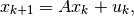
with $A=\left[\begin{array}{cc}\cos 1 & -\sin 1\\ \sin 1 & \cos 1\end{array}\right]$ , $\ u_k \in \{u\in {\bf R}^2 ~|~ \|u\|_{\infty}\leqslant1\}$ , and $x_0 \in \{x\in {\bf R}^2 ~|~ \|x\|_{\infty}\leqslant1\}$ .

Starting with a rectangular initial set, the number of vertices of the reach set polytope is $4k + 4$ at the $k$ th step.

In $d/dt$ [DDTHP], the reach set is approximated by unions of rectangular polytopes [ASAR2000].

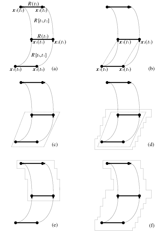
Figure 14: Reach set approximation by union of rectangles. Source: adapted from [ASAR2000].

The algorithm works as follows. First, given the set of initial conditions defined as a polytope, the evolution in time of the polytope’s extreme points is computed (figure 14 (a)).

$R(t_1)$ in figure 14 (a) is the reach set of the system at time $t_1$ , and $R[t_0, t_1]$ is the set of all points that can be reached during $[t_0, t_1]$ . Second, the algorithm computes the convex hull of vertices of both, the initial polytope and $R(t_1)$ (figure 14 (b)). The resulting polytope is then bloated to include all the reachable states in $[t_0,t_1]$ (figure 14 (c)). Finally, this overapproximating polytope is in its turn overapproximated by the union of rectangles (figure 14 (d)). The same procedure is repeated for the next time interval $[t_1,t_2]$ , and the union of both rectangular approximations is taken (figure 14 (e,f)), and so on. Rectangular polytopes are easy to represent and the number of facets grows linearly with dimension, but a large number of rectangles must be used to assure the approximation is not overly conservative. Besides, the important part of this method is again the convex hull calculation whose implementation relies on the same CDD/CDD+ library. This limits the dimension of the system and time interval for which it is feasible to calculate the reach set.

Polytopes can give arbitrarily close approximations to any convex set, but the number of vertices can grow prohibitively large and, as shown in [AVIS1997], the computation of a polytope by its convex hull becomes intractable for large number of vertices in high dimensions.

The method of zonotopes for approximation of reach sets ([GIR2005], [GIR2006], [MATHP]) uses a special class of polytopes (see [ZONOHP]) of the form,

$Z=\{x \in {\bf R}^n ~|~ x=c+\sum_{i=1}^p\alpha_ig_i,~ -1\leqslant\alpha_i\leqslant1\},$

wherein $c$ and $g_1, ..., g_p$ are vectors in ${\bf R}^n$ . Thus, a zonotope $Z$ is represented by its center $c$ and ‘generator’ vectors $g_1, ..., g_p$ . The value $p/n$ is called the order of the zonotope. The main benefit of zonotopes over general polytopes is that a symmetric polytope can be represented more compactly than a general polytope. The geometric sum of two zonotopes is a zonotope:

$Z(c_1, G_1)\oplus Z(c_2, G_2) = Z(c_1+c_2, [G_1 ~ G_2]),$

wherein $G_1$ and $G_2$ are matrices whose columns are generator vectors, and $[G_1 ~ G_2]$ is their concatenation. Thus, in the reach set computation, the order of the zonotope increases by $p/n$ with every time step. This difficulty can be averted by limiting the number of generator vectors, and overapproximating zonotopes whose number of generator vectors exceeds the limit by lower order zonotopes. The benefits of the compact zonotype representation, however, appear to diminish because in order to plot them or check if they intersect with given objects and compute those intersections, these operations are performed after converting zonotopes to polytopes.

CheckMate [CMHP] is a Matlab toolbox that can evaluate specifications for trajectories starting from the set of initial (continuous) states corresponding to the parameter values at the vertices of the parameter set. This provides preliminary insight into whether the specifications will be true for all parameter values. The method of oriented rectangluar polytopes for external approximation of reach sets is introduced in [STUR2003]. The basic idea is to construct an oriented rectangular hull of the reach set for every time step, whose orientation is determined by the singular value decomposition of the sample covariance matrix for the states reachable from the vertices of the initial polytope. The limitation of CheckMate and the method of oriented rectangles is that only autonomous (i.e. uncontrolled) systems, or systems with fixed input are allowed, and only an external approximation of the reach set is provided.

All the methods described so far employ the notion of time step, and calculate the reach set or its approximation at each time step. This approach can be used only with discrete-time systems. By contrast, the analytic methods which we are about to discuss, provide a formula or differential equation describing the (continuous) time evolution of the reach set or its approximation.

The level set method ([MIT2000], [LSTHP]) deals with general nonlinear controlled systems and gives exact representation of their reach sets, but requires solving the HJB equation and finding the set of states that belong to sub-zero level set of the value function. The method [LSTHP] is impractical for systems of dimension higher than three.

Requiem [REQHP] is a Mathematica notebook which, given a linear system, the set of initial conditions and control bounds, symbolically computes the exact reach set, using the experimental quantifier elimination package. Quantifier elimination is the removal of all quantifiers (the universal quantifier $\forall$ and the existential quantifier $\exists$ ) from a quantified system. Each quantified formula is substituted with quantifier-free expression with operations $+$ , $\times$ , $=$ and $<$ . For example, consider the discrete-time system

$x_{k+1} = Ax_k + Bu_k$

with $A=\left[\begin{array}{cc}0 & 1\\0 & 0\end{array}\right]$ and $B=\left[\begin{array}{c}0\\1\end{array}\right]$ .

For initial conditions $x_0\in\{x\in {\bf R}^2 ~|~ \|x\|_{\infty} \leqslant1\}$ and controls $u_k\in\{u\in {\bf R} ~|~ -1\leqslant u\leqslant1\}$ , the reach set for $k\geqslant0$ is given by the quantified formula

$\{ x\in{\bf R}^2 ~|~ \exists x_0, ~~ \exists k\geqslant0, ~~ \exists u_i, ~ 0\leqslant i\leqslant k: ~~ x = A^kx_0+\sum_{i=0}^{k-1}A^{k-i-1}Bu_i \},$

which is equivalent to the quantifier-free expression

$-1\leqslant[1 ~~ 0]x\leqslant1 ~ \wedge ~ -1\leqslant[0 ~~ 1]x\leqslant1.$

It is proved in [LAFF2001] that for continuous-time systems, $\dot{x}(t) = Ax(t) + Bu(t)$ , if $A$ is constant and nilpotent or is diagonalizable with rational real or purely imaginary eigenvalues, and with suitable restrictions on the control and initial conditions, the quantifier elimination package returns a quantifier free formula describing the reach set. Quantifier elimination has limited applicability.

The reach set approximation via parallelotopes [KOST2001] employs the idea of parametrization described in [KUR2000] for ellipsoids. The reach set is represented as the intersection of tight external, and the union of tight internal, parallelotopes. The evolution equations for the centers and orientation matrices of both external and internal parallelotopes are provided. This method also finds controls that can drive the system to the boundary points of the reach set, similarly to [VAR1998] and [KUR2000]. It works for general linear systems. The computation to solve the evolution equation for tight approximating parallelotopes, however, is more involved than that for ellipsoids, and for discrete-time systems this method does not deal with singular state transition matrices.

Ellipsoidal Toolbox (ET) implements in MATLAB the ellipsoidal calculus [KUR1997] and its application to the reachability analysis of continuous-time [KUR2000], discrete-time [VAR2007], possibly time-varying linear systems, and linear systems with disturbances [KUR2001], for which ET calculates both open-loop and close-loop reach sets. The ellipsoidal calculus provides the following benefits:

The complexity of the ellipsoidal representation is quadratic in the dimension of the state space, and linear in the number of time steps.
It is possible to exactly represent the reach set of linear system through both external and internal ellipsoids.
It is possible to single out individual external and internal approximating ellipsoids that are optimal to some given criterion (e.g. trace, volume, diameter), or combination of such criteria.
We obtain simple analytical expressions for the control that steers the state to a desired target.

The report is organized as follows. Chapter 2 describes the operations of the ellipsoidal calculus: affine transformation, geometric sum, geometric difference, intersections with hyperplane, ellipsoid, halfspace and polytope, calculation of maximum ellipsoid, calculation of minimum ellipsoid. Chapter 3 presents the reachability problem and ellipsoidal methods for the reach set approximation. Chapter 4 contains Ellipsoidal Toolbox installation and quick start instructions, and lists the software packages used by the toolbox. Chapter 5 describes structures and objects implemented and used in toolbox. Also it describes the implementation of methods from chapters 2 and 3 and visualization routines. Chapter 6 describes structures and objects implemented and used in the toolbox. Chapter 6 gives examples of how to use the toolbox. Chapter 7 collects some conclusions and plans for future toolbox development. The functions provided by the toolbox together with their descriptions are listed in appendix A.

References

[MOTZ1953]

T. S. Motzkin, H. Raiffa, G. L. Thompson, and R. M. Thrall. The double description method. In H. W. Kuhn and A. W. Tucker, editors, Conttributions to Theory of Games, volume 2. Princeton University Press, 1953.

[CDDHP]

CDD/CDD+ homepage. http://www.cs.mcgill.ca/~fukuda/soft/cdd_home/cdd.html.

[DDTHP]

$d/dt$ homepage. http://www-verimag.imag.fr/~tdang/ddt.html.

[ASAR2000]

(1, 2) E.Asarin, O.Bournez, T.Dang, and O.Maler. Approximate reachability analysis of piecewise linear dynamical systems. In N.Lynch and B.H.Krogh, editors, Hybrid Systems: Computation and Control, volume 1790 of Lecture Notes in Computer Science, pages 482–497. Springer, 2000.

[AVIS1997]

D. Avis, D. Bremner, and R. Seidel. How good are convex hull algorithms? Computational Geometry: Theory and Applications, 7:265–301, 1997.

[GIR2005]

A. Girard. Reachability of uncertain linear systems using zonotopes. In M. Morari, L. Thiele, and F. Rossi, editors, Hybrid Systems: Computation and Control, volume 3414 of Lecture Notes in Computer Science, pages 291–305. Springer, 2005.

[GIR2006]

A.Girard, C.Le Guernic, and O.Maler. Computation of reachable sets of linear time-invariant systems with inputs. In J.Hespanha and A.Tiwari, editors, Hybrid Systems: Computation and Control, volume 3927 of Lecture Notes in Computer Science, pages 257–271. Springer, 2006.

[MATHP]

MATISSE homepage. http://www.seas.upenn.edu/~agirard/Software/MATISSE.

[ZONOHP]

Zonotope methods on Wolfgang Kühn homepage. http://www.decatur.de.

[CMHP]

CheckMate homepage. http://www.ece.cmu.edu/~webk/checkmate.

[STUR2003]

O. Stursberg and B. H. Krogh. Efficient representation and computation of reachable sets for hybrid systems. In O. Maler and A. Pnueli, editors, Hybrid Systems: Computation and Control, volume 2623 of Lecture Notes in Computer Science, pages 482–497. Springer, 2003.

[MIT2000]

I. Mitchell and C. Tomlin. Level set methods for computation in hybrid systems. In N. Lynch and B. H. Krogh, editors, Hybrid Systems: Computation and Control, volume 1790 of Lecture Notes in Computer Science, pages 21–31. Springer, 2000.

[LSTHP]

(1, 2) Level Set Toolbox homepage. http://www.cs.ubc.ca/~mitchell/ToolboxLS.

[REQHP]

Requiem homepage. http://www.seas.upenn.edu/~hybrid/requiem/requiem.html.

[LAFF2001]

G. Lafferriere, G. J. Pappas, and S. Yovine. Symbolic reachability computation for families of linear vector fields. Journal of Symbolic Computation, 32:231–253, 2001.

[KOST2001]

E. K. Kostousova. Control synthesis via parallelotopes: optimization and parallel computations. Optimization Methods and Software, 14(4):267–310, 2001.

[KUR2000]

(1, 2, 3) A. B. Kurzhanski and P. Varaiya. On ellipsoidal techniques for reachability analysis. Optimization Methods and Software, 17:177–237, 2000.

[VAR1998]

P. Varaiya. Reach set computation using optimal control. Proc. of KITWorkshop on Verification on Hybrid Systems. Verimag, Grenoble., 1998.

[KUR1997]

A. B. Kurzhanski and I. Vályi. Ellipsoidal Calculus for Estimation and Control. ser. SCFA. Birkhäuser, 1997.

[KUR2001]

A. B. Kurzhanski and P. Varaiya. Reachability analysis for uncertain systems - the ellipsoidal technique. Dynamics of Continuous, Discrete and Impulsive Systems Series B: Applications and Algorithms, 9:347–367, 2001.

Introduction¶

References

Previous topic

Next topic

This Page

Navigation

Introduction¶

References

Previous topic

Next topic

This Page

Quick search

Navigation