Implementation
Operations with ellipsoids
In the Ellipsoidal Toolbox we define a new class ellipsoid inside the
MATLAB programming environment. The following three commands define the
same ellipsoid  , with
  and
and
 being symmetric positive semidefinite:
1 2 3 4 5 | centVec = [1 2]';
shMat = eye(2, 2);
ellObj = ellipsoid(centVec, shMat);
ellObj = ellipsoid(shMat) + centVec;
ellObj = sqrtm(shMat)*ell_unitball(size(shMat, 1)) + centVec;
|
For the ellipsoid class we overload the following functions and operators:
- isEmpty(ellObj) - checks if is an empty
ellipsoid.
- display(ellObj) - displays the details of ellipsoid
, namely, its center
 and the shape
matrix
and the shape
matrix  .
. - plot(ellObj) - plots ellipsoid if its
dimension is not greater than 3.
- firstEllObj == secEllObj - checks if ellipsoids
 and
and  are
equal.
are
equal. - firstEllObj ~= secEllObj - checks if ellipsoids
and are
not equal.
- [ , ] - concatenates the ellipsoids into the horizontal array, e.g. ellVec = [firstEllObj secEllObj thirdEllObj].
- [ ; ] - concatenates the ellipsoids into the vertical array, e.g. ellMat =
[firstEllObj secEllObj; thirdEllObj fourthEllObj] defines
 array of ellipsoids.
 - firstEllObj >= secEllObj - checks if the ellipsoid firstEllObj is
bigger than the ellipsoid secEllObj, or equivalently
 .
. - firstEllObj <= secEllObj - checks if
 .
. - -ellObj - defines ellipsoid
 .
. - ellObj + bScal - defines ellipsoid
 .
. - ellObj - bScal - defines ellipsoid
 .
. - aMat * ellObj - defines ellipsoid
 .
. - ellObj.inv() - inverts the shape matrix of the ellipsoid:
 .
.
All the listed operations can be applied to a single ellipsoid as well as to a two-dimensional array of ellipsoids. For example,
1 2 3 4 5 6 7 8 9 10 11 12 13 14 | % nondegenerate ellipsoid in R^2
firstEllObj = ellipsoid([2; -1], [9 -5; -5 4]);
secEllObj = firstEllObj.polar();% secEll is polar ellipsoid for firstEllObj
% thirdEllObj is generated from secEllObj by inverting its shape matrix
thirdEllObj = secEllObj.getInv();
% 2x2 array of ellipsoids
ellMat = [firstEllObj secEllObj; thirdEllObj ellipsoid([1; 1], eye(2))];
% check if firstEllObj is bigger than each of the ellipsoids in ellMat
ellMat <= firstEllObj
% ans =
%
% 1 0
% 1 0
|
To access individual elements of the array, the usual MATLAB subindexing is used:
1 2 3 4 | aMat = [0 1; -2 0]; % aMat - 2x2 real matrix
bVec = [3; 0]; % bVec - vector in R^2
% affine transformation of ellipsoids in the second column of ellMat
aTransMat = aMat * ellMat(:, 2) + bVec;
|
Sometimes it may be useful to modify the shape of the ellipsoid without affecting its center. Say, we would like to bloat or squeeze the ellipsoid:
1 2 | bltEllObj = firstEllObj.getShape(2); % bloats ellipsoid firstEllObj
sqzEllObj = firstEllObj.getShape(0.5); % squeezes ellipsoid firstEllObj
|
Since function shape does not change the center of the ellipsoid, it only accepts scalars or square matrices as its second input parameter. Several functions access the internal data of the ellipsoid object:
1 2 3 4 5 6 7 8 9 10 | [centVec, shMat] = secEllObj.double()
% centVec =
%
% -0.5000
% -0.1667
%
% shMat =
%
% 0.9167 0.9167
% 0.9167 1.5278
|
1 2 3 4 5 6 7 8 | % define new ellipsoid
fourthEllObj = ellipsoid([42 -7 -2 4; -7 10 3 1; -2 3 5 -2; 4 1 -2 2]);
bufEllVec = [ellMat(1, :) fourthEllObj];
bufEllVec.isdegenerate() % check if given ellipsoids are degenerate
% ans =
%
% 0 0 1
|
1 2 3 4 5 6 7 8 9 10 11 | bufEllVec = [ellMat(1, :) fourthEllObj];
[dimVec, rankVec] = bufEllVec.dimension()
% dimVec =
%
% 2 2 4
%
% rankVec =
%
% 2 2 3
|
One way to check if two ellipsoids intersect, is to compute the distance between them ([STANHP], [LIN2002]):
1 2 3 4 5 6 7 | % distance between thirdEllObj and each of the ellipsoids in ellMat
ellMat.distance(thirdEllObj)
% ans =
%
% 0 0
% 0 0.1683
|
This result indicates that the ellipsoid thirdEllObj does not intersect with the ellipsoid ellMat(2, 2), with all the other ellipsoids in ellMat it has nonempty intersection. If the intersection of the two ellipsoids is nonempty, it can be approximated by ellipsoids from the outside as well as from the inside. See [ROS2002] for more information about these methods.
1 2 3 4 | % external approximation of intersection of firstEllObj and thirdEllObj
externalEllObj = firstEllObj.intersection_ea(thirdEllObj);
% internal approximation of intersection of firstEllObj and thirdEllObj
internalEllObj = firstEllObj.intersection_ia(thirdEllObj);
|
It can be checked that resulting ellipsoid externalEllObj contains the given intersection, whereas internalEllObj is contained in this intersection:
1 2 3 4 5 6 | % array [firstEllObj secEllObj] should be treated as intersection
externalEllObj.doesIntersectionContain([firstEllObj secEllObj], 'i')
% ans =
%
% 1
|
1 2 3 4 5 6 | bufEllVec = [firstEllObj thirdEllObj]
bufEllVec.doesIntersectionContain(internalEllObj)
% ans =
%
% 1
|
Function isInside in general checks if the intersection of ellipsoids in the given array contains the union or intersection of ellipsoids or polytopes.
It is also possible to solve the feasibility problem, that is, to check if the intersection of more than two ellipsoids is empty:
1 2 3 4 5 | ellMat.intersect(ellMat(1, 1), 'i')
% ans =
%
% -1
|
In this
particular example the result  indicates that the intersection
of ellipsoids in ellMat is empty. Function intersect in general checks
if an ellipsoid, hyperplane or polytope intersects the union or the
intersection of ellipsoids in the given array:
indicates that the intersection
of ellipsoids in ellMat is empty. Function intersect in general checks
if an ellipsoid, hyperplane or polytope intersects the union or the
intersection of ellipsoids in the given array:
1 2 3 4 5 6 | bufEllVec = [firstEllObj secEllObj thirdEllObj]
bufEllVec.intersect(ellMat(2, 2), 'i')
% ans =
%
% 0
|
1 2 3 4 5 6 | bufEllVec = [firstEllObj secEllObj thirdEllObj];
bufEllVec.intersect(ellMat(2, 2), 'u')
% ans =
%
% 1
|
For the ellipsoids in
 ,
,  and
and  the geometric
sum can be computed explicitely and plotted:
the geometric
sum can be computed explicitely and plotted:
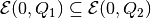
1 | ellMat.minksum();
|
Figure 8: The geometric sum of ellipsoids.
Figure 8 displays the geometric sum of ellipsoids. If
the dimension of the space in which the ellipsoids are defined exceeds
 , an error is returned. The result of the geometric sum
operation is not generally an ellipsoid, but it can be approximated by
families of external and internal ellipsoids parametrized by the
direction vector:
, an error is returned. The result of the geometric sum
operation is not generally an ellipsoid, but it can be approximated by
families of external and internal ellipsoids parametrized by the
direction vector:
1 2 3 4 5 6 7 8 9 10 11 12 13 14 15 16 17 18 19 20 21 22 | % define the set of directions:
% columns of matrix dirsMat are vectors in R^2
dirsMat = [1 0; 1 1; 0 1; -1 1; 1 3]';
% compute external ellipsoids for the directions in dirsMat
externalEllVec = ellMat.minksum_ea(dirsMat)
% externalEllVec =
% Array of ellipsoids with dimensionality 1x5
% compute internal ellipsoids for the directions in dirsMat
internalEllVec = ellMat.minksum_ia(dirsMat)
% internalEllVec =
% Array of ellipsoids with dimensionality 1x5
% intersection of external ellipsoids should always contain
% the union of internal ellipsoids:
externalEllVec.doesIntersectionContain(internalEllVec, 'u')
%
% ans =
%
% 1
|
Functions minksum_ea and minksum_ia work for ellipsoids of arbitrary dimension. They should be used for general computations whereas minksum is there merely for visualization purposes.
If the geometric difference of two ellipsoids is not an empty set, it
can be computed explicitely and plotted for ellipsoids in
, and :
1 2 3 4 5 6 7 8 9 10 11 | % ellipsoid defined by squeezing the ellipsoid ellMat(2, 2)
fourthEllObj = ellMat(2, 2).getShape(0.4);
% check if the geometric difference firstEllObj - fourthEllObj is nonempty
firstEllObj >= fourthEllObj
%
% ans =
%
% 1
% compute and plot this geometric difference
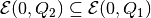
firstEllObj.minkdiff(fourthEllObj);
|
Figure 9: The geometric difference of ellipsoids.
Figure 9 shows the geometric difference of ellipsoids.
Similar to minksum, minkdiff is there for visualization purpose. It
works only for dimensions  ,
,  and , and for
higher dimensions it returns an error. For arbitrary dimensions, the
geometric difference can be approximated by families of external and
internal ellipsoids parametrized by the direction vector, provided this
direction is not bad:
and , and for
higher dimensions it returns an error. For arbitrary dimensions, the
geometric difference can be approximated by families of external and
internal ellipsoids parametrized by the direction vector, provided this
direction is not bad:
1 2 3 4 5 6 7 8 9 10 11 12 13 14 15 16 17 18 19 20 21 | absTol = getAbsTol(firstEllObj);
% find out which of the directions in dirsMat are bad
firstEllObj.isbaddirection(fourthEllObj, dirsMat, absTol)
% ans =
%
% 1 0 0 1 0
% two of five directions specified by dirsMat are bad,
% so, only three ellipsoidal approximations
% can be produced for this dirsMat:
externalEllVec = firstEllObj.minkdiff_ea(fourthEllObj, dirsMat)
% externalEllVec =
% Array of ellipsoids with dimensionality 1x3
internalEllVec = firstEllObj.minkdiff_ia(fourthEllObj, dirsMat)
% internalEllVec =
% Array of ellipsoids with dimensionality 1x3
|
Operation ’difference-sum’ described in section
2.2.4 is implemented in functions minkmp, minkmp_ea, minkmp_ia, the
first one of which is used for visualization and works for dimensions
not higher than , whereas the last two can deal with ellipsoids
of arbitrary dimension.
1 2 3 4 5 6 7 8 9 10 11 12 13 14 | % ellipsoidal approximations for (firstEllObj - thirdEllObj + secEllObj)
% external
externalEllVec = firstEllObj.minkmp_ea(thirdEllObj, secEllObj, dirsMat)
% externalEllVec =
% Array of ellipsoids with dimensionality 1x5
% internal
internalEllVec = firstEllObj.minkmp_ia(thirdEllObj, secEllObj, dirsMat)
% internalEllVec =
% Array of ellipsoids with dimensionality 1x5
% plot the set (firstEllObj - thirdEllObj + secEllObj)
firstEllObj.minkmp(thirdEllObj, secEllObj, 'newfigure', true);
|
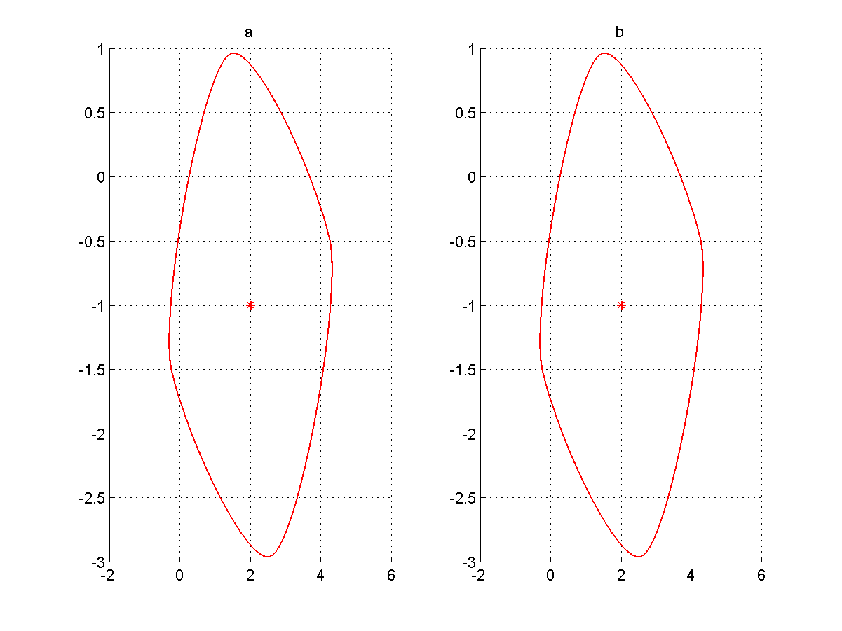
Figure 10: Implementation of operations ‘sum-difference’ and ‘difference-sum’.
Figure 10 displays results of the implementation of minkpm and minkmp operations.
Similarly, operation ’sum-difference’ described in section Geometric Sum-Difference is implemented in functions
minkpm, minkpm_ea, minkpm_ia, the first one of which is used for
visualization and works for dimensions not higher than ,
whereas the last two can deal with ellipsoids of arbitrary dimension.
1 2 3 4 5 6 7 8 9 10 11 12 13 14 | % ellipsoidal approximations for (firstEllObj + secEllObj - thirdEllObj)
bufEllVec = [firstEllObj secEllObj];
externalEllVec = bufEllVec.minkpm_ea(thirdEllObj, dirsMat) % external
% externalEllVec =
% Array of ellipsoids with dimensionality 1x5
internalEllVec = bufEllVec.minkpm_ia(thirdEllObj, dirsMat) % internal
% internalEllVec =
% Array of ellipsoids with dimensionality 1x4
% plot the set (firstEllObj + secEllObj - thirdEllObj)
firstEllObj.minkpm(secEllObj, thirdEllObj, 'newfigure', true)
|
Operations with hyperplanes
The class hyperplane of the Ellipsoidal Toolbox is used to describe hyperplanes and halfspaces. The following two commands define one and the same hyperplane but two different halfspaces:
1 2 | firstHypObj = hyperplane([1; 1], 1); % defines halfspace x1 + x2 <= 1
firstHypObj = hyperplane([-1; -1], -1); % defines halfspace x1 + x2 >= 1
|
The following functions and operators are overloaded for the hyperplane class:
- isempty(hypObj) – checks if hypObj is an empty hyperplane.
- display(hypObj) – displays the details of hyperplane
 , namely, its normal
  and the scalar
 .
. - plot(hypObj) – plots hyperplane if the dimension
of the space in which it is defined is not greater than 3.
- firstHypObj == secHypObj – checks if hyperplanes
 and
and  are equal.
 - firstHypObj = secHypObj – checks if hyperplanes
and are not equal.
- [ , ] – concatenates the hyperplanes into the horizontal array, e.g. hypVec = [firstHypObj secHypObj thirdHypObj].
- [ ; ] – concatenates the hyperplanes into the vertical array, e.g. hypMat =
[firstHypObj secHypObj; thirdHypObj fourthHypObj] – defines
array of hyperplanes.
- -hypObj – defines hyperplane
 , which is the same
as but specifies different halfspace.
, which is the same
as but specifies different halfspace.
There are several ways to access the internal data of the hyperplane object:
1 2 3 4 5 6 7 8 9 10 | [normVec, hypScal] = firstHypObj.double()
% normVec =
%
% -1
% -1
%
% hypScal =
%
% -1
|
1 2 3 4 5 | firstHypObj.dimension()
% ans =
%
% 2
|
1 2 3 4 5 6 7 | % define two hyperplanes passing through the origin
secHypObj = hyperplane([1 -1; 1 1]);
firstHypObj.isparallel(secHypObj)
% ans =
%
% 1 0
|
All the functions of Ellipsoidal Toolbox that accept hyperplane object as parameter, work with single hyperplanes as well as with hyperplane arrays. One exception is the function parameters that allows only single hyperplane object.
An array of hyperplanes can be converted to the polytope object of the Multi-Parametric Toolbox ([KVAS2004], [MPTHP]), and back:
1 2 3 4 5 6 7 8 9 10 11 12 13 14 15 16 17 18 19 20 21 22 23 24 25 26 27 28 29 30 31 32 33 34 35 36 37 38 39 40 41 42 43 44 45 46 47 48 49 50 51 52 53 54 55 56 57 58 | %define array of four hyperplanes:
hypVec = hyperplane([1 1; -1 -1; 1 -1; -1 1]', [2 2 2 2])
% array of hyperplanes:
% size: [1 4]
%
% Element: [1 1]
% Normal:
% 1
% 1
%
% Shift:
% 2
%
% Hyperplane in R^2.
%
%
% Element: [1 2]
% Normal:
% -1
% -1
%
% Shift:
% 2
%
% Hyperplane in R^2.
%
%
% Element: [1 3]
% Normal:
% 1
% -1
%
% Shift:
% 2
%
% Hyperplane in R^2.
%
%
% Element: [1 4]
% Normal:
% -1
% 1
%
% Shift:
% 2
%
% Hyperplane in R^2.
% convert array of hyperplanes to polytope
firstPolObj = hyperplane2polytope(hypVec);
% covert polytope to array of hyperplanes
convertedHypVec = polytope2hyperplane(firstPolObj);
convertedHypVec == hypVec
% ans =
%
% 1 1 1 1
|
Functions hyperplane2polytope and polytope2hyperplane require the Multi-Parametric Toolbox to be installed.
We can compute distance from ellipsoids to hyperplanes and polytopes:
1 2 3 4 5 6 7 8 9 10 11 12 13 14 15 | % distance from ellipsoid firstEllObj to each of the hyperplanes in hypVec
firstEllObj.distance(hypVec)
% ans =
%
% -0.5176 0.8966 -2.6841 0.1444
% distance from each of the ellipsoids in ellMat to the polytope
% firstPolObj
ellMat.distance(firstPolObj)
% ans =
%
% 0 0
% 0 0
|
A negative distance value in the case of ellipsoid and hyperplane means that the ellipsoid intersects the hyperplane. As we see in this example, ellipsoid firstEllObj intersects hyperplanes hypVec(1) and hypVec(3) and has no common points with hypVec(2) and hypVec(4). When distance function has a polytope as a parameter, it always returns nonnegative values to be consistent with distance function of the Multi-Parametric Toolbox. Here, the zero distance values mean that each ellipsoid in ellMat has nonempty intersection with polytope firstPolObj.
It can be checked if the union or intersection of given ellipsoids intersects given hyperplanes or polytopes:
1 2 3 4 5 | ellMat.intersect(hypVec, 'u')
% ans =
%
% 1 1 1 1
|
1 2 3 4 5 | ellMat(:, 1).intersect(hypVec, 'i')
% ans =
%
% 0 0 1 0
|
1 2 3 4 5 6 | bufEllVec = [firstEllObj secEllObj thirdEllObj];
bufEllVec.intersect(firstPolObj, 'i')
% ans =
%
% 1
|
The intersection of ellipsoid and hyperplane can be computed exactly:
1 2 3 4 5 6 7 8 9 10 11 12 13 14 | % compute the intersections of ellipsoids in the second column of ellMat
% with hyperplane firstHypObj:
intersectEllMat = ellMat(:, 2).hpintersection(firstHypObj)
% intersectEllMat =
% Array of ellipsoids with dimensionality 2x1
intersectEllMat.isdegenerate() % resulting ellipsoids should lose rank
% ans =
%
% 1
% 1
|
Functions intersection_ea and intersection_ia can be used with hyperplane objects, which in this case define halfspaces and polytope objects:
1 2 3 4 5 6 7 8 9 10 11 12 13 14 15 16 17 18 19 20 21 22 23 24 25 26 27 28 29 30 | % compute external and internal ellipsoidal approximations
% of the intersections of ellipsoids in the first column of ellMat
% with the halfspace x1 - x2 <= 2:
% get external ellipsoids
firstExternalEllMat = ellMat(:, 1).intersection_ea(firstHypObj(1))
% firstExternalEllMat =
% Array of ellipsoids with dimensionality 2x1
% get internal ellipsoids
firstInternalEllMat = ellMat(:, 1).intersection_ia(firstHypObj(1))
% firstInternalEllMat =
% Array of ellipsoids with dimensionality 2x1
% compute external and internal ellipsoidal approximations
% of the intersections of ellipsoids in the first column of ellMat
% with the halfspace x1 - x2 >= 2:
% get external ellipsoids
secExternalEllMat = ellMat(:, 1).intersection_ea(-firstHypObj(1));
% get internal ellipsoids
secInternalEllMat = ellMat(:, 1).intersection_ia(-firstHypObj(1));
% compute ellipsoidal approximations of the intersection
% of ellipsoid firstEll and polytope firstPol:
% get external ellipsoid
externalEllMat = ellMat(:, 1).intersection_ea(firstPolObj);
% get internal ellipsoid
internalEllMat = ellMat(:, 1).intersection_ia(firstPolObj);
|
Function isInside can be used to check if a polytope or union of polytopes is contained in the intersection of given ellipsoids:
1 2 3 4 5 6 7 8 9 10 11 12 | % polytope secPolObj is obtained by affine transformation of firstPolObj
secPolObj = 0.5*firstPolObj + [1; 1];
% check if the intersection of ellipsoids in the first column of ellMat
% contains the union of polytopes firstPolObj and secPolObj:
% equivalent to: doesIntersectionContain(ellMat(:, 1), firstPolObj | secPolObj)
ellMat(:, 1).doesIntersectionContain([firstPolObj secPolObj])
% ans =
%
% 0
|
1 2 3 4 5 6 7 | % equivalent to: doesIntersectionContain(ellMat(2, 2),...
% firstPolObj & secPolObj)
ellMat(2, 2).doesIntersectionContain([firstPolObj secPolObj], 'i')
% ans =
%
% 1
|
Functions distance, intersect, intersection_ia and isInside use the CVX interface ([CVXHP]) to the external optimization package. The default optimization package included in the distribution of the Ellipsoidal Toolbox is SeDuMi ([STUR1999], [SDMHP]).
Operations with ellipsoidal tubes
There are several classes in Ellipsoidal Toolbox for operations with ellipsoidal tubes. The class gras.ellapx.smartdb.rels.EllTube is used to describe ellipsoidal tubes. The class gras.ellapx.smartdb.rels.EllUnionTube is used to store tubes by the instant of time:
(1)![{\mathcal X}_{U}[t]=\bigcup \limits_{\tau\leqslant t}{\mathcal X}[\tau],](_images/math/53ca07410d079433f63db3afd5fd5ba975724616.png)
where ![{\mathcal X}[\tau]](_images/math/456d10b00ec6c948f7306d194e252da674e291d1.png) is single ellipsoidal tube. The class
gras.ellapx.smartdb.rels.EllTubeProj is used to describe the projection
of the ellipsoidal tubes onto time dependent subspaces.There are two
types of projection: static and dynamic. Also there is class
gras.ellapx.smartdb.rels.EllUnionTubeStaticProj for description of the
projection on static plane tubes by the instant of time. Next we provide
some examples of the operations with ellipsoidal tubes.
is single ellipsoidal tube. The class
gras.ellapx.smartdb.rels.EllTubeProj is used to describe the projection
of the ellipsoidal tubes onto time dependent subspaces.There are two
types of projection: static and dynamic. Also there is class
gras.ellapx.smartdb.rels.EllUnionTubeStaticProj for description of the
projection on static plane tubes by the instant of time. Next we provide
some examples of the operations with ellipsoidal tubes.
1 2 3 4 5 6 7 8 9 10 11 12 13 14 15 16 17 | nPoints=5;
absTol=0.001;
relTol=0.001;
approxSchemaDescr=char.empty(1,0);
approxSchemaName=char.empty(1,0);
nDims=3;
nTubes=1;
lsGoodDirVec=[1;0;1];
aMat=zeros(nDims,nPoints);
timeVec=1:nPoints;
sTime=nPoints;
approxType=gras.ellapx.enums.EApproxType.Internal;
qArrayList=repmat({repmat(diag([1 2 3]),[1,1,nPoints])},1,nTubes);
ltGoodDirArray=repmat(lsGoodDirVec,[1,nTubes,nPoints]);
fromMatEllTube=gras.ellapx.smartdb.rels.EllTube.fromQArrays(qArrayList,...
aMat, timeVec,ltGoodDirArray, sTime, approxType,...
approxSchemaName, approxSchemaDescr, absTol, relTol);
|
1 2 3 4 5 6 7 8 9 10 | ellArray(nPoints) = ellipsoid();
approxType=gras.ellapx.enums.EApproxType.Internal;
sTime= 2;
for iElem = 1:nPoints
ellArray(iElem) = ellipsoid(...
aMat(:,iElem), qArrayList{1}(:,:,iElem));
end
fromEllArrayEllTube = gras.ellapx.smartdb.rels.EllTube.fromEllArray(...
ellArray, timeVec,ltGoodDirArray, sTime, approxType,...
approxSchemaName,approxSchemaDescr, absTol, relTol);
|
We may be
interested in the data about ellipsoidal tube in some particular time
interval, smaller than the one for which the ellipsoidal tube was
computed, say  . This data can be extracted
by the cut function:
. This data can be extracted
by the cut function:
1 2 | cutTimeVec = [2, 4];
cutEllTube = fromMatEllTube.cut(cutTimeVec);
|
1 2 3 4 5 6 7 8 9 10 11 12 13 14 15 16 17 18 19 20 21 22 23 24 25 26 27 28 29 30 | function example
aMat = [0 1; 0 0]; bMat = eye(2);
SUBounds = struct();
SUBounds.center = {'sin(t)'; 'cos(t)'};
SUBounds.shape = [9 0; 0 2];
sys = elltool.linsys.LinSysContinuous(aMat, bMat, SUBounds);
x0EllObj = ell_unitball(2);
timeVec = [0 10];
dirsMat = [1 0; 0 1]';
rsObj = elltool.reach.ReachContinuous(sys, x0EllObj, dirsMat, timeVec);
ellTubeObj = rsObj.getEllTubeRel();
projSpaceList = {[1 0;0 1]};
projType = gras.ellapx.enums.EProjType.Static;
statEllTubeProj = ellTubeObj.project(projType,projSpaceList,...
@fGetProjMat);
projType = gras.ellapx.enums.EProjType.DynamicAlongGoodCurve;
dynEllTubeProj=ellTubeObj.project(projType,projSpaceList,...
@fGetProjMat);
plObj=smartdb.disp.RelationDataPlotter();
statEllTubeProj.plot(plObj);
dynEllTubeProj.plot(plObj);
end
function [projOrthMatArray,projOrthMatTransArray]=fGetProjMat(projMat,...
timeVec,varargin)
nTimePoints=length(timeVec);
projOrthMatArray=repmat(projMat,[1,1,nTimePoints]);
projOrthMatTransArray=repmat(projMat.',[1,1,nTimePoints]);
end
|
We can compute the projection of the ellipsoidal tube onto time-dependent subspace.
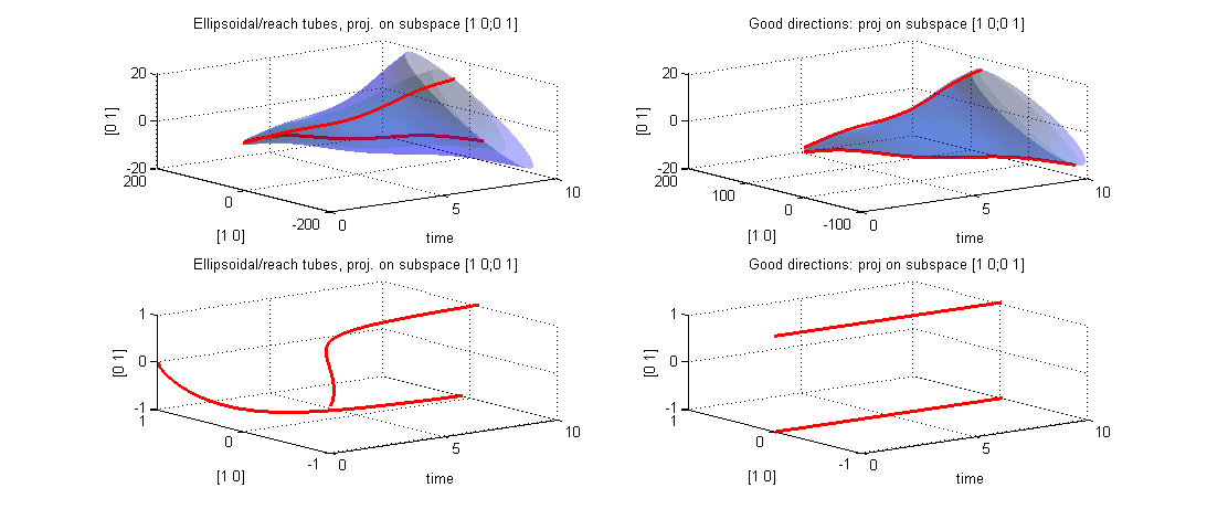
Figure 11: Static and dynamic projections of the ellipsoidal tube.
Figure 11 displays static and dynamic projections. Also we can see projections of good directions for ellipsoidal tubes.
We can compute tubes by the instant of time using methodfromEllTubes:
1 2 3 4 5 6 7 8 9 10 11 12 13 14 15 16 17 18 19 20 21 22 23 24 25 26 27 | function example
aMat = [0 1; 0 0]; bMat = eye(2);
SUBounds = struct();
SUBounds.center = {'sin(t)'; 'cos(t)'};
SUBounds.shape = [9 0; 0 2];
sys = elltool.linsys.LinSysContinuous(aMat, bMat, SUBounds);
x0EllObj = ell_unitball(2);
timeVec = [0 10];
dirsMat = [1 0; 0 1]';
rsObj = elltool.reach.ReachContinuous(sys, x0EllObj, dirsMat, timeVec);
ellTubeObj = rsObj.getEllTubeRel();
unionEllTube = ...
gras.ellapx.smartdb.rels.EllUnionTube.fromEllTubes(ellTubeObj);
projSpaceList = {[1 0;0 1]};
projType = gras.ellapx.enums.EProjType.Static;
statEllTubeProj = unionEllTube.project(projType,projSpaceList,...
@fGetProjMat);
plObj=smartdb.disp.RelationDataPlotter();
statEllTubeProj.plot(plObj);
end
function [projOrthMatArray,projOrthMatTransArray]=fGetProjMat(projMat,...
timeVec,varargin)
nTimePoints=length(timeVec);
projOrthMatArray=repmat(projMat,[1,1,nTimePoints]);
projOrthMatTransArray=repmat(projMat.',[1,1,nTimePoints]);
end
|
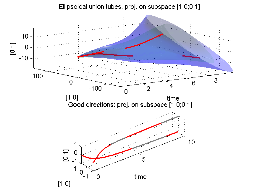
Figure 12: Ellipsoidal tubes by the instant of time.
Figure 12 shows projection of ellipsoidal tubes by the instant of time.
Also we can get initial data from the resulting tube:
1 2 3 4 5 | approxType=gras.ellapx.enums.EApproxType.Internal;
ellArray = fromEllArrayEllTube.getEllArray(approxType)
% ellArray =
% Array of ellipsoids with dimensionality 5x1
|
There is a method to display a content of ellipsoidal tubes.
1 2 3 4 5 6 7 8 9 10 11 12 13 14 15 | aMat = [0 1; 0 0]; bMat = eye(2);
SUBounds = struct();
SUBounds.center = {'sin(t)'; 'cos(t)'};
SUBounds.shape = [9 0; 0 2];
sys = elltool.linsys.LinSysContinuous(aMat, bMat, SUBounds);
x0EllObj = ell_unitball(2);
timeVec = [0 10];
for iElem = 1:5
dirInitial= rand(2, 1);
dirInitial = dirInitial ./ norm(dirInitial);
dirsMat(:, iElem) = dirInitial;
end
rsObj = elltool.reach.ReachContinuous(sys, x0EllObj, dirsMat, timeVec);
ellTubeObj = rsObj.getEllTubeRel();
ellTubeObj.dispOnUI();
|
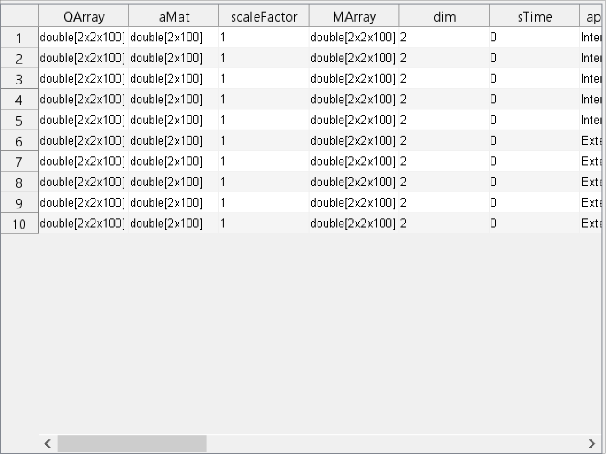
Figure 13: Content of the ellipsoidal tube.
Figure 13 displays all fields of the ellipsoidal tube.
There are several methods to find the tubes with necessary parameters.
1 2 3 4 5 6 7 8 9 10 11 12 13 14 | newEllTube = fromMatEllTube.getTuplesFilteredBy('sTime', 5);
newEllTube.getNTuples()
%
% ans =
%
% 1
%
newEllTube = fromMatEllTube.getTuplesFilteredBy('sTime', 2);
newEllTube.getNTuples()
%
% ans =
%
% 0
%
|
Also you can use the method display to see the result of the method’s work.
1 2 3 4 5 6 7 8 9 10 11 12 13 14 15 16 17 18 19 20 21 22 23 24 25 26 27 28 29 30 31 32 | fromMatEllTube.getNTuples()
%
% ans =
%
% 1
%
fromEllArrayEllTube.getNTuples()
%
% ans =
%
% 1
%
origFromMatEllTube=fromMatEllTube.getCopy();
fromMatEllTube.unionWith(fromEllArrayEllTube);
%
% ans =
%
% 2
%
fromMatEllTube.getNTuples()
isOk=fromMatEllTube.getTuples(1).isEqual(origFromMatEllTube)
%
% isOk =
%
% 1
isOk=fromMatEllTube.getTuples(2).isEqual(fromEllArrayEllTube)
%
% isOk =
%
% 1
|
We can sort our tubes by certain fields:
1 2 3 | fromMatEllTube.display();
fromMatEllTube.sortBy('sTime');
fromMatEllTube.display();
|
Reachability
To compute the reach sets of the systems described in chapter 3, we
define few new classes in the Ellipsoidal Toolbox: class
LinSysContinuous for the continuous-time system description, class
LinSysDiscrete for the discrete-time system description and classes
ReachContinuous ReachDiscrete for the reach set
data. We start by explaining how to define a system using
LinSysContinuous object. Also we can use LinSysFactory class for the
description of this system. Through it’s method create user can get
LinSysContinuous or LinSysDiscrete object. For example, description of
the system
ReachDiscrete for the reach set
data. We start by explaining how to define a system using
LinSysContinuous object. Also we can use LinSysFactory class for the
description of this system. Through it’s method create user can get
LinSysContinuous or LinSysDiscrete object. For example, description of
the system
![\left[\begin{array}{cc}
\dot{x}_1\\
\dot{x}_2\end{array}\right] = \left[\begin{array}{cc}
0 & 1\\
0 & 0\end{array}\right]\left[\begin{array}{c}
x_1\\
x_2\end{array}\right] + \left[\begin{array}{c}
u_1(t)\\
u_2(t)\end{array}\right], ~~~ u(t)\in{\mathcal E}(p(t), P)](_images/math/b0af0118992b1d96f54dee81d0a8db0ea5f99e5d.png)
with
![p(t) = \left[\begin{array}{c}
\sin(t)\\
\cos(t)\end{array}\right], ~~~ P = \left[\begin{array}{cc}
9 & 0\\
0 & 2\end{array}\right],](_images/math/9c916c53b1e7ef1d576998bd08de918790ec7770.png)
is done by the following sequence of commands:
1 2 3 4 5 6 7 8 | aMat = [0 1; 0 0]; bMat = eye(2); % matrices A and B, B is identity
SUBounds = struct();
% center of the ellipsoid depends on t
SUBounds.center = {'sin(t)'; 'cos(t)'};
SUBounds.shape = [9 0; 0 2]; % shape matrix of the ellipsoid is static
% create linear system object
sys = elltool.linsys.LinSysContinuous(aMat, bMat, SUBounds);
% is equal to sys = elltool.linsys.LinSysFactory.create(aMat, bMat, SUBounds)
|
If matrices  or
or
 depend on time, say
 ![A(t)=\left[\begin{array}{cc}
0 & 1-\cos(2t)\\
-\frac{1}{t} & 0\end{array}\right]](_images/math/eec5acb8455659ea4d7044850d9494b15a460658.png) , then matrix aMat should be
symbolic:
, then matrix aMat should be
symbolic:
1 2 | atMat = {'0' '1 - cos(2*t)'; '-1/t' '0'};
sys_t = elltool.linsys.LinSysFactory.create(atMat, bMat, SUBounds);
|
To describe the system with disturbance
![\left[\begin{array}{cc}
\dot{x}_1\\
\dot{x}_2\end{array}\right] = \left[\begin{array}{cc}
0 & 1\\
0 & 0\end{array}\right]\left[\begin{array}{c}
x_1\\
x_2\end{array}\right] + \left[\begin{array}{c}
u_1(t)\\
u_2(t)\end{array}\right] + \left[\begin{array}{c}
0\\
1\end{array}\right]v(t),](_images/math/41225beced2d5270cd3d2e7ec57ad88e66576a6d.png)
with bounds on control as before, and disturbance being
 , we type:
1 2 3 4 | gMat = [0; 1]; % matrix G
vEllObj = ellipsoid(1); % disturbance bounds: unit ball in R
sys_d = elltool.linsys.LinSysContinuous(aMat, bMat, SUBounds,...
gMat, vEllObj);
|
Control and disturbance bounds SUBounds and vEllObj can have different types. If the bound is constant, it should be described by ellipsoid object. If the bound depends on time, then it is represented by a structure with fields center and shape, one or both of which are symbolic. In system sys, the control bound SUBounds is defined as such a structure. Finally, if the control or disturbance is known and fixed, it should be defined as a vector, of type double if constant, or symbolic, if it depends on time.
To declare a discrete-time system
![\left[\begin{array}{c}
x_1[k+1]\\
x_2[k+1]\end{array}\right] = \left[\begin{array}{cc}
0 & 1\\
-1 & -0.5\end{array}\right]\left[\begin{array}{c}
x_1[k]\\
x_2[k]\end{array}\right] + \left[\begin{array}{c}
0\\
1\end{array}\right]u[k], ~~~ -1\leqslant u[k]\leqslant1,](_images/math/da2c3d0815dc2cf770cf3c1c7aa0b91fe0da37ab.png)
we use LinSysDiscrete constructor:
1 2 3 4 5 6 | adMat = [0 1; -1 -0.5]; bdMat = [0; 1]; % matrices A and B
udBoundsEllObj = ellipsoid(1); % control bounds: unit ball in R
% discrete-time system
dtsys = elltool.linsys.LinSysDiscrete(adMat, bdMat, udBoundsEllObj);
% is equal to dtsys = elltool.linsys.LinSysFactory.create(adMat, bdMat,...
% udBoundsEllObj,...[], [], [], [], 'd');
|
Once the LinSysDiscrete object is created, we need to specify the set of initial conditions, the time interval and values of the direction vector, for which the reach set approximations must be computed:
1 2 3 | x0EllObj = ell_unitball(2); % set of initial conditions
timeVec = [0 10]; % time interval
dirsMat = [1 0; 0 1]'; % columns of L specify the directions
|
The reach set approximation is computed by calling the constructor of the ReachContinuous object:
1 2 | % reach set of continuos-time system
firstRsObj = elltool.reach.ReachContinuous(sys, x0EllObj, dirsMat, timeVec);
|
At this point, variable firstRsObj contains the reach set approximations for the specified continuous-time system, time interval and set of initial conditions computed for given directions. Both external and internal approximations are computed. The reach set approximation data can be extracted in the form of arrays of ellipsoids:
1 2 3 4 5 6 7 | externallEllMat = firstRsObj.get_ea() % external approximating ellipsoids
% externallEllMat =
% Array of ellipsoids with dimensionality 2x100
% internal approximating ellipsoids
[internalEllMat, timeVec] = firstRsObj.get_ia();
|
Ellipsoidal arrays externallEllMat and internalEllMat have  rows because we computed the reach set approximations for
directions. Each row of ellipsoids corresponds to one direction. The
number of columns in externallEllMat and internalEllMat is defined by
the nTimeGridPoints parameter, which is available from
elltool.conf.Properties static class (see chapter 6 for details). It
represents the number of time values in our time interval, at which the
approximations are evaluated. These time values are returned in the
optinal output parameter, array timeVec, whose length is the same as the
number of columns in externallEllMat and internalEllMat. Intersection of
ellipsoids in a particular column of externallEllMat gives external
ellipsoidal approximation of the reach set at corresponding time.
Internal ellipsoidal approximation of this set at this time is given by
the union of ellipsoids in the same column of internalEllMat.
rows because we computed the reach set approximations for
directions. Each row of ellipsoids corresponds to one direction. The
number of columns in externallEllMat and internalEllMat is defined by
the nTimeGridPoints parameter, which is available from
elltool.conf.Properties static class (see chapter 6 for details). It
represents the number of time values in our time interval, at which the
approximations are evaluated. These time values are returned in the
optinal output parameter, array timeVec, whose length is the same as the
number of columns in externallEllMat and internalEllMat. Intersection of
ellipsoids in a particular column of externallEllMat gives external
ellipsoidal approximation of the reach set at corresponding time.
Internal ellipsoidal approximation of this set at this time is given by
the union of ellipsoids in the same column of internalEllMat.
We may be interested in the reachability data of our system in some
particular time interval, smaller than the one for which the reach set
was computed, say  . This data can be
extracted and returned in the form of ReachContinuous object by the cut
function:
. This data can be
extracted and returned in the form of ReachContinuous object by the cut
function:
1 | cutObj = firstRsObj.cut([3 5]); % reach set for the time interval [3, 5]
|
To obtain a snap shot of the reach set at given time, the same function cut is used:
1 | cutObj = firstRsObj.cut(5); % reach set at time t = 5
|
It can be checked if the external or internal reach set approximation intersects with given ellipsoids, hyperplanes or polytopes:
1 2 3 4 5 6 7 8 9 10 | ellObj = ellipsoid([-17; 0], [4 -1; -1 1]); % define ellipsoid
% define 4 hyperplanes
hypVec = hyperplane([1 1; -1 -1; 1 -1; -1 1]', [2 2 2 2]);
polObj = hyperplane2polytope(hypVec) + [2; 10]; % define polytope
% check if ellipsoid ell intersects with external approximation:
cutObj.intersect(ellObj, 'e')
% ans =
%
% 1
|
1 2 3 4 5 6 7 | % check if ellipsoid ellObj intersects with internal approximation:
cutObj.intersect(ellObj, 'i')
%
% ans =
%
% 1
|
1 2 3 4 5 6 | % check if hyperplanes in hypVec intersect with internal approximation:
cutObj.intersect(hypVec, 'i')
% ans =
%
% 1 1 1 1
|
1 2 3 4 5 6 | % check if polytope polObj intersects with external approximation:
cutObj.intersect(polObj)
% ans =
%
% 0
|
If a given set intersects with the internal approximation of the reach set, then this set intersects with the actual reach set. If the given set does not intersect with external approximation, this set does not intersect the actual reach set. There are situations, however, when the given set intersects with the external approximation but does not intersect with the internal one. In our example above, ellipsoid ellObj is such a case: the quality of the approximation does not allow us to determine whether or not ellObj intersects with the actual reach set. To improve the quality of approximation, refine function should be used:
1 2 3 4 5 6 7 8 9 10 11 12 | % define new directions, in this case one, but could be more
newDirsMat = [1; -1];
% compute approximations for the new directions
firstRsObj = firstRsObj.refine(newDirsMat);
% snap shot of the reach set at time t = 5
cutObj = firstRsObj.cut(5);
% check if ellObj intersects the internal approximation
cutObj.intersect(ellObj, 'i')
% ans =
%
% 1
|
Now we are sure that ellipsoid ellObj intersects with the actual reach set. However, to use the refine function, the reach set object must contain all calculated data, otherwise, an error is returned.
Having a reach set object resulting from the ReachContinuous, cut or refine operations, we can obtain the trajectory of the center of the reach set and the good curves along which the actual reach set is touched by its ellipsoidal approximations:
1 2 3 4 5 | [ctrMat, ttVec] = firstRsObj.get_center(); % trajectory of the center
gcCVec = firstRsObj.get_goodcurves() % get good curves
% gcCVec =
% [2x100 double] [2x100 double] [2x100 double]
|
Variable ctrMat here is a matrix whose columns are the points ofthe
reach set center trajectory evaluated at time values returned in the
array ttVec. Variable gcCMat contains matrices each of which
corresponds to a good curve (columns of such matrix are points of the
good curve evaluated at time values in ttVec). The analytic expression
for the control driving the system along a good curve is given by
formula.
We computed the reach set up to time  . It is possible to
continue the reach set computation for a longer time horizon using the
reach set data at time as initial condition. It is also
possible that the dynamics and inputs of the system change at certain
time, and from that point on the system evolves according to the new
system of differential equations. For example, starting at time
, our reach set may evolve in time according to the
time-variant system sys_t defined above. Switched systems are a special
case of this situation. To compute the further evolution in time of the
existing reach set, function evolve should be used:
. It is possible to
continue the reach set computation for a longer time horizon using the
reach set data at time as initial condition. It is also
possible that the dynamics and inputs of the system change at certain
time, and from that point on the system evolves according to the new
system of differential equations. For example, starting at time
, our reach set may evolve in time according to the
time-variant system sys_t defined above. Switched systems are a special
case of this situation. To compute the further evolution in time of the
existing reach set, function evolve should be used:
1 2 3 4 5 6 7 8 9 10 | % reach set from time 10 to 14 with the same dynamics
secRsObj = firstRsObj.evolve(14);
% reach set from time 10 to 12 with new dynamics
secRsObj = firstRsObj.evolve(12, sys_t);
% not only the dynamics, but the inputs can change as well,
% from time 12 to 13 disturbance is added to the system:
% sys_d - system with disturbance defined above
thirdRsObj = secRsObj.evolve(13, sys_d);
|
Function evolve can be viewed as an implementation of the semigroup property.
To compute the backward reach set for some specified target set, we declare the time interval so that the terminating time comes first:
1 2 3 4 5 6 7 8 9 | % target set in the form of ellipsoid
yEllObj = ellipsoid([8; 2], [4 1; 1 2]);
tbTimeVec = [10 5]; % backward time interval
% backward reach set
firstBrsObj = elltool.reach.ReachContinuous(sys, yEllObj, dirsMat,...
tbTimeVec);
firstBrsObj = firstBrsObj.refine(newDirsMat); % refine the approximation
% further evolution in backward time from 5 to 0;
secBrsObj = firstBrsObj.evolve(0)
|
Reach set and backward reach set computation for discrete-time systems and manipulations with the resulting reach set object are performed using the same functions as for continuous-time systems:
1 2 3 4 5 6 7 8 9 10 11 12 13 14 15 16 | timeVec = [0 100]; % represents 100 time steps from 1 to 100
% reach set for 100 time steps
secDtrsObj = elltool.reach.ReachDiscrete(dtsys, x0EllObj, dirsMat, timeVec);
secDtrsObj = secDtrsObj.evolve(200); % compute next 100 time steps
tbTimeVec = [50 0]; % backward time interval
% backward reach set
dtbrsObj = elltool.reach.ReachDiscrete(dtsys, yEllObj, dirsMat, tbTimeVec);
dtbrsObj = dtbrsObj.refine(newDirsMat); % refine the approximation
% get external approximating ellipsoids and time values
[externallEllMat, timeVec] = dtbrsObj.get_ea();
% get internal approximating ellipsoids
internalEllMat = dtbrsObj.get_ia()
% internalEllMat =
% Array of ellipsoids with dimensionality 3x51
|
Number of columns in the ellipsoidal arrays externalEllMat and
internalEllMat is  because the backward reach set is computed
for
because the backward reach set is computed
for  time steps, and the first column of these arrays contains
ellipsoids yEllObj - the terminating condition.
time steps, and the first column of these arrays contains
ellipsoids yEllObj - the terminating condition.
When dealing with discrete-time systems, all functions that accept time or time interval as an input parameter, round the time values and treat them as integers.
Properties
Functions of the Ellipsoidal Toolbox can be called with user-specified values of certain global parameters. System of the parameters are configured using xml files, which available from a set of command-line utilities:
1 | elltool.setconf('default');
|
Here we list system parameters available from the ’default’ configuration:
- version = ’1.4dev’ - current version of ET.
- isVerbose = false - makes all the calls to ET routines silent, and no information except errors is displayed.
- absTol = 1e-7 - absolute tolerance.
- relTol = 1e-5 - relative tolerance.
- nTimeGridPoints = 200 - density of the time grid for the continuous
time reach set computation. This parameter directly affects the
number of ellipsoids to be stored in the
ReachContinuousReachDiscrete object.
- ODESolverName = ode45 - specifies the ODE solver for continuous time reach set computation.
- isODENormControl = ’on’ - switches on and off the norm control in the ODE solver. When turned on, it slows down the computation, but improves the accuracy.
- isEnabledOdeSolverOptions = false - when set to false, calls the ODE solver without any additional options like norm control. It makes the computation faster but less accurate. Otherwise, it is assumed to be true, and only in this case the previous option makes a difference.
- nPlot2dPoints = 200 - the number of points used to plot a 2D ellipsoid. This parameter also affects the quality of 2D reach tube and reach set plots.
- nPlot3dPoints = 200 - the number of points used to plot a 3D ellipsoid. This parameter also affects the quality of 3D reach set plots.
Once the configuration is loaded, the system parameters are available through elltool.conf.Properties. elltool.conf.Properties is a static class, providing emulation of static properties for toolbox. It has two function types: setters and getters. Using getters we obtain system parameters.
1 2 3 4 5 6 7 8 9 10 | elltool.conf.Properties.getAbsTol()
% ans =
%
% 1.0000e-07
elltool.conf.Properties.getNPlot2dPoints()
% ans =
%
% 200
|
Some of the parameters can be changed in run-time via setters.
1 | elltool.conf.Properties.setNTimeGridPoints(250);
|
Visualization
Ellipsoidal Toolbox has several plotting routines:
- ellipsoid/plot - plots one or more ellipsoids, or arrays of
ellipsoids, defined in , or
.
- ellipsoid/minksum - plots geometric sum of finite number of
ellipsoids defined in , or
.
- ellipsoid/minkdiff - plots geometric difference (if it is not an
empty set) of two ellipsoids defined in ,
or .
- ellipsoid/minkmp - plots geometric (Minkowski) sum of the geometric
difference of two ellipsoids and the geometric sum of
 ellipsoids defined in , or
.
ellipsoids defined in , or
. - ellipsoid/minkpm - plots geometric (Minkowski) difference of the
geometric sum of ellipsoids and a single ellipsoid defined in
, or .
- hyperplane/plot - plots one or more hyperplanes, or arrays of
hyperplanes, defined in or .
- reach/plot_ea - plots external approximation of the reach set whose
dimension is or .
- reach/plot_ia - plots internal approximation of the reach set whose
dimension is or .
All these functions allow the user to specify the color of the plotted objects, line width for 1D and 2D plots, and transparency level of the 3D objects. Hyperplanes are displayed as line segments in 2D and square facets in 3D. In the hyperplane/plot method it is possible to specify the center of the line segment or facet and its size.
Ellipsoids of dimensions higher than three must be projected onto a two- or three-dimensional subspace before being plotted. This is done by means of projection function:
1 2 3 4 5 6 7 8 9 10 11 12 13 14 15 16 17 18 | % create two 4-dimensional ellipsoids:
firstEllObj = ellipsoid([14 -4 2 -5; -4 6 0 1; 2 0 6 -1; -5 1 -1 2]);
secEllObj = firstEllObj.getInv();
% specify 3-dimensional subspace by its basis:
% columns of basisMat must be orthogonal
basisMat = [1 0 0 0; 0 0 1 0; 0 1 0 1].';
% get 3-dimensional projections of firstEllObj and secEllObj:
bufEllVec = [firstEllObj secEllObj];
% array ellVec contains projections of firstEllObj and secEllObj
ellVec = bufEllVec.projection(basisMat)
% ellVec =
% Array of ellipsoids with dimensionality 1x2
ellVec.plot(); % plot ellipsoids in ellVec
|
Since the operation of projection is linear, the projection of the geometric sum of ellipsoids equals the geometric sum of the projected ellipsoids. The same is true for the geometric difference of two ellipsoids.
Function projection exists also for the
ReachContinuousReachDiscrete objects:
1 2 3 4 5 6 7 8 9 10 11 12 13 14 15 16 | aMat = [0 1 0 0; -1 0 1 0; 0 0 0 1; 0 0 -1 0];
bMat = [0; 0; 0; 1];
uBoundsEllObj = ellipsoid(1);
% 4-dimensional system
sys = elltool.linsys.LinSysFactory.create(aMat, bMat, uBoundsEllObj);
dirsMat = [1 1 0 1; 0 -1 1 0; -1 1 1 1; 0 0 -1 1].'; % matrix of directions
% reach set from time 0 to 5
rsObj = elltool.reach.ReachContinuous(sys, ell_unitball(4), dirsMat,...
[0 5], 'isRegEnabled', true, 'isJustCheck', false, 'regTol', 1e-4);
basisMat = [1 0 0 1; 0 1 1 0].'; % basis of 2-dimensional subspace
% project reach set rs onto basis basisMat
psObj = rsObj.projection(basisMat);
psObj.plotByEa(); % plot external approximation
hold on;
psObj.plotByIa(); % plot internal approximation
|
The quality of the ellipsoid and reach set plots is controlled by the parameters nPlot2dPoints and nPlot3dPoints, which are available from getters of ellipsoid class.
References
| [STANHP] | Stanley Chan Article Homepage. http://videoprocessing.ucsd.edu/~stanleychan/publication/unpublished/Ellipse.pdf. |
| [LIN2002] | Lin A., and S. Han. 2002. On the Distance Between Two Ellipsoids. SIAM Journal on Optimization 13 (1): 298–308. |
| [KVAS2004] | M. Kvasnica, P. Grieder, M. Baotic, and M. Morari. Multi-Parametric Toolbox (MPT). In R. Alur and G. J. Pappas, editors, Hybrid Systems: Computation and Control, volume 2993 of Lecture Notes in Computer Science, pages 448–462. Springer, 2004. |